4. Training the model: a minimal batch app

Now that we have our data ready, the next goal is to setup a process to fetch the records, train and evaluate a regression model and deploy it to perform predictions. In this chapter we will review how to create a bare minimal app to do it using a Jupyter notebook, also covering how to deploy the notebook in docker container to have an executable app.

4.1. Writing the notebook

Similar to when we were loading data into Carol, to fetch data we have also to start by making a connection to Carol feeding our credentials. As our goal is to run the code inside a batch app we can skip the full authentication and use the simplified version.

from pycarol import Carol, Staging, ApiKeyAuth

''' Complete authentication for tests running locally
# =================== AUTHENTICATION ON CAROL ===================
# Paste here your connection id and token
connectors = {"mltutorial": '0f0883dXX2434057XXXf07ef86eXXXXX'}
conn_tokens = {"mltutorial": '906XXb5ae5e7413c97fXXXX7d0XXXXXX'}
# ===============================================================

login = Carol(domain="mltutorial",
                            app_name="bostonhouseprice",
                            organization='datascience',
                            auth=ApiKeyAuth(conn_tokens["mltutorial"]),
                            connector_id=connectors["mltutorial"])
'''

#Simplified version for when running it inside an carol app
login = Carol()

We then consume the data directly from staging with the code below. Data will be returned from the fecth_parquet function as a dataframe. The latest parameters available to the function are up to date in the code documentation.

# Buiding a staging object on top of the login credentials
staging = Staging(login)

# Defining the connector and staging where the data should be accessed
conn = "boston_house_price"
stag = "samples"

# Specifying the columns to be used
X_cols = ["CRIM", "ZN", "INDUS", "CHAS", "NOX", "RM", "AGE", "DIS", "RAD", "TAX", "PTRATIO", "B", "LSTAT"]
y_col = ["target"]
roi_cols = X_cols + y_col

# Fecthing data from Carol
data = staging.fetch_parquet(staging_name=stag,
                                                         connector_name=conn,
                                                         cds=True,
                                                         columns=roi_cols)

In this example we use a very simple training process just to ilustrate the goal: split the data into a training and testing parts and fit a Multilayer Perceptron (MLPRegressor), with default parameters, on the training set.

from sklearn.model_selection import train_test_split
from sklearn.neural_network import MLPRegressor

# Splitting the dataset: 80% for training, 20% for test
X_train, X_test, y_train, y_test = train_test_split(data[X_cols],
                                                    data[y_col],
                                                    test_size=0.20,
                                                    random_state=1,
                                                                                                        shuffle=True)

# Fitting a standard hyperparameters MLP regressor
mlp_model = MLPRegressor(random_state=1, max_iter=500)
mlp_model.fit(X_train,
                            y_train["target"].values)

We then evaluate our model against the test set using the classical regression evaluation metrics MSE, MAE and RMSE.

import numpy as np

# Calculating the error (residuals)
y_real = list(y_test["target"].values)
residual = list(y_test["target"].values) - y_pred

# Calculating summary metrics
mse_f = np.mean(residual**2)
mae_f = np.mean(abs(residual))
rmse_f = np.sqrt(mse_f)

# Printing the results
display(f"Mean Squared Error (MSE): {mse_f}.")
display(f"Mean Absolute Error (MAE): {mae_f}.")
display(f"Root Mean Squared Error (RMSE): {rmse_f}.")

# Results
'''
Mean Squared Error (MSE): 32.83513021826763.
Mean Absolute Error (MAE): 4.538316218898927.
Root Mean Squared Error (RMSE): 5.7301946056192214.
'''

We can also evaluate our regression in further details by plotting a residual scatter plot. The residual plot allows us to check the error distribution along different values of y.

import pandas as pd
import seaborn as sns; sns.set_theme(color_codes=True)
from matplotlib import pyplot as plt

# Organize the real values and the predictions on a dataframe
res_df = pd.DataFrame({"y":y_real, "res":residual})

# Make the plot on a 20 by 8 panel
plt.figure(figsize=(20,8))
ax = sns.regplot(x="y", y="res", data=res_df)

# Add legends
ax.set_title('Residual Plot')
tmp = ax.set(xlabel='Real Value', ylabel='Prediction Error')

The resulting plot is presented on figure 19.

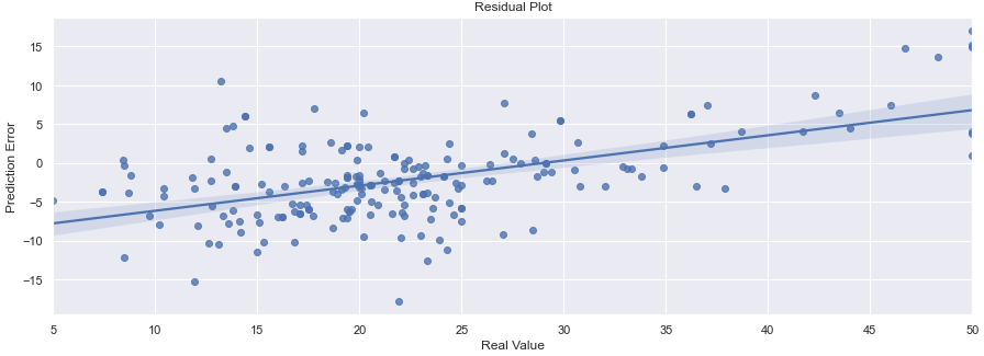
Figure 19: The residual plot achieved by the MLP model we trained

If from the evaluation we conclude the model is good enough to our needs, we can deploy it by saving it to the local storage. The code is given below.

# Saving the model to the storage.
stg = Storage(login)
stg.save("bhp_mlp_regressor", mlp_model, format='pickle')

With the code snippet above you are publishing the model as pickle file to the storage on the same app you are running. If you are interested in deploying your model somewhere else (an online app, for example), you can simply change the login variable and point it to the correct app.

# Authenticating on Carol with default parameters from the enviornment
login = Carol()

# Pointing to a different application under the same environment
login.app_name = 'my_online_app'

# Pointing to a different application in a different environment and org level
login.switch_environment(org_name="another_org_level",
                                                 env_name="another_environment",
                                                 app_name='my_online_app')

In some situations you may be interested in publishing the model to an app in another environment, perhaps even in a different organization level. In that case you can use the switch_environment method. One of the advantages is that access control will be managed automatically: if the user running the process has access granted to the target environment the process will run smothly, otherwise the batch will fail with denied authentication.

The whole code is available at this github repo.

4.2. Files for the batch app

Apart from the code, there are a couple of other files which we need to revise to be able to build our app inside Carol, they are:

requirements.txt: This file is nothing but a list of modules used in our application.
manifest.json: Brings definitions on how the app needs to be built and how it will run.
Dockerfile: Sets the docker commands necessary to build the app.

Starting with requirements.txt, we want to fill it with the python modules on the list below. During the build docker will asure we have these libs installed on the environment, you can also enforce the lib version as in pandas==1.2.5. This is a way of fixing problems with new releases and grant the app behaves the same way no matter which environment it is deployed.

pycarol[complete]
sklearn
runipy
seaborn

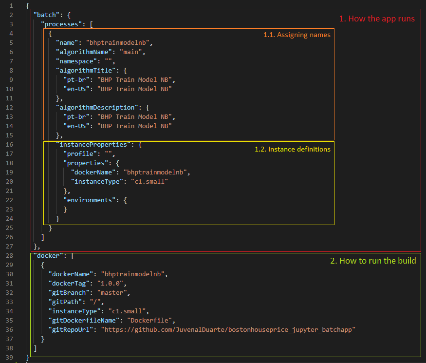
In the manifest.json there are two main sections, the first defining how the app runs (1) and the second defining how it is built (2). For the namings on (1.1) the only caution is that algorithmTitle and algorithmDescriptionfields accept any string, while name allows only lowercased strings without spaces or special characters.

../../imgs/tutorial_ch4\_fig2.png — ../../imgs/tutorial_ch4_fig2.png

Figure 19: Main sections on the manifest.json file

On the instanceProperties section (1.2) we define on which type of cloud instance and which parameters to use when running the app. The first important field is property/dockerName, which should follow the following standard:

"dockerName": "yourcarolappname"

Next you define the size of the machine you want to use when executing your code on property/instanceType. A complete list of instance types available are covered in the official documentation, at this link.

On the docker section (2) we set the necessary configurations needed to build our app. The fields are:

dockerName: The name of the docker container where the code is going to run. For convention we set it as the same name in batch/process/name, lowercased and without spaces or special characters.
dockerTag: Used for version control.
gitRepoUrl: To build the app all the files need to be placed at a version control repository. The link to the repository must be provided in this field.
gitBranch: The version control branch where the files resides.
gitPath: Use / when the Dockerfile is on the root path or the corresponding path otherwise.
instanceType: The cloud machine used to build the code.
gitDockerfileName: The docker file name on your repository.

The final mandatory file is the Dockerfile (or any other name depending on the definition on gitDockerfileName). In this file we have a sequence of commands necessary to make sure the environment has the right files, the right base software and the right lib versions to run the code without conflicts. A full description of how to construct the file is given on the official docker manual, at this link.

For our minimal batch app we will use the Dockerfile as below:

# Setting the base cloud image to be enhanced
FROM totvslabs/pycarol:2.40.0

# Copying the requirement file and installing the dependencies
RUN mkdir /app
WORKDIR /app
ADD requirements.txt /app/
RUN pip install -r requirements.txt

# Configuring the entry point for the app
ADD . /app
CMD ["runipy", "bhp_trainmodel.ipynb"]

Together with the notebook, the final setup on git should be as in:

https://github.com/totvslabs/pyCarol/tree/master/tutorial/chapters/ch4_basic_batchapp.

4.3. Deploying to Carol

The only remaining step now is to deploy our app in Carol, so that we can run it whenever we want with a single click. We start by creating a new app through the UI, as in figure 20.

Note: pay attention at this point and make sure the name you assign to your app corresponds to the same used on the manifest.json file, on property/dockerName.

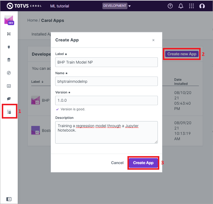
Figure 20: Creating an App on Carol to deploy our code.

Now select the File tab, click on Upload File button, select the manifest.json file we’ve created previously and then click on Open(figure 21).

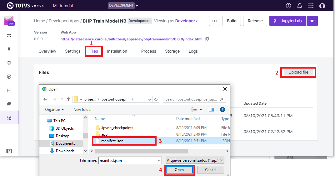
Figure 21: Loading the manifest file to the platform.

The manifest.json already puts together everything we need for the build. The files and the code will be retrieved from the version control repository pointed in gitRepoUrl.

To run the build click on the Build button, the next screen will ask you for your github token (figure 22). The github token allows Carol the fetch the files from your github account, for the specified branch. You can follow the steps on the official documentation to generate a new github token.

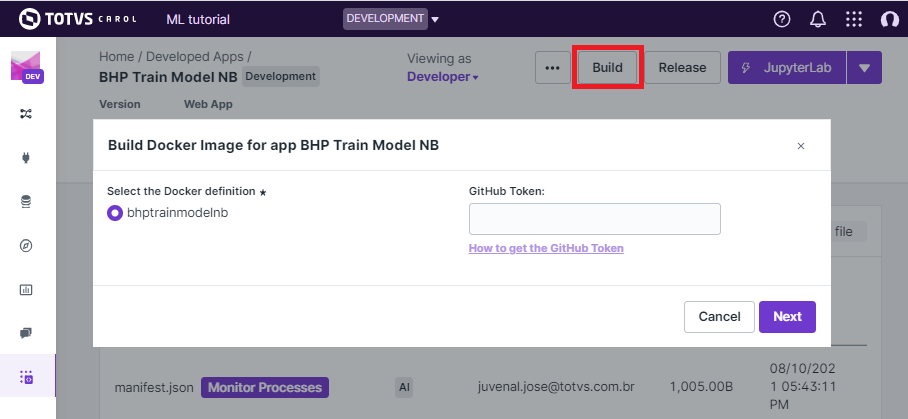
Figure 22: Build: providing the github token

On the next screen just make sure your app version and instance type for the build are correct, then click on Build Image.

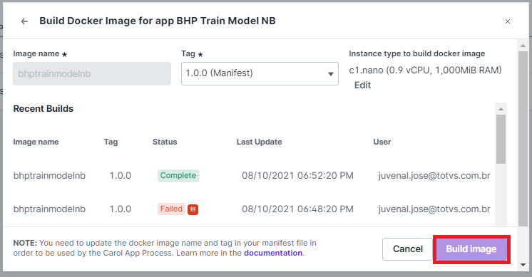
Figure 23: Revising and running the buid.

The process for building the app usually takes from 5 to 15 minutes to perform the setup. If everything goes well you will see the screen on figure 24.

Figure 24: Image successfully built

4.4. Running the app

On the Process tab on your app’s panel, there are two ways of setting up a execution for your app, as pointed on figure 25: (1) Run it manually by clicking on the Run button; (2) Schedule single or recurrent executions through the Add a Schedule option.

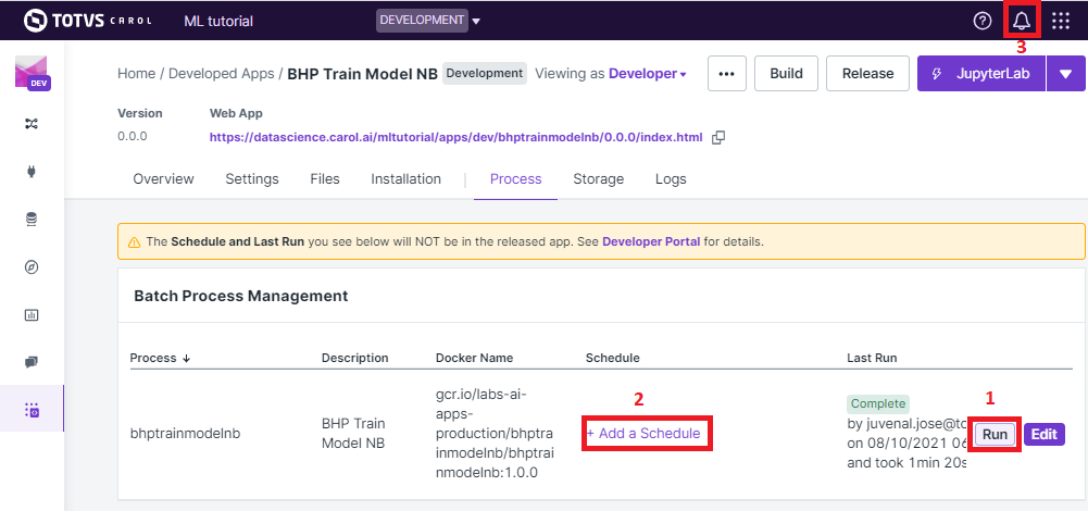
Figure 25: Running your app

Once started a pop-up screen will open informing you on whether the process is still running, concluded or have failed. You can also check detailed info about the process and other tasks on the small bell icon on the top right of the screen (check (3) on figure 25).

Finally, the Logs tab on the app’s panel will print the output of your code. Remember to mantain your app’s verbosity at a reasonable level.

4.5. Troubleshooting

Below are are presented some well known problems when developing/ deploying Carol Apps:

``instanceType`` is not big enough: Correctly sizing resources is essential to control costs when running apps. On the other hand, if the process is memory or CPU intensive, your process may run out of resources either on build or on execution. For the build it is common to run out of memory if dependencies include heavy packages, such as pytorch, requiring at least c1.small (5Gb RAM).
Wrong ``gitRepoUrl``, ``gitBranch`` or ``gitPath``: When handling big repositories you can easily get confused and end up building the wrong version of your code. Another subtle problem is that recent github repositories use master to refer to the head branch, while old ones refer as main.
The docker container doesn’t replicates all the environment files / libs as on local tests: We often run on the situation where tests work fine on the local machine, but fails when running it remotely. Docker containers aim to help with such problems, but to do so the build process must be well defined. If you are reading any file from your local disk, make sure this file is also deployed together on your build. If you are using a lib with constant updates, make sure to explicitly set the lib version on your requirements to the same version on your local machine.
Code issues: Code issues rarely impacts the building process, but they usually arises when running the app. Several type of issues may arise when running the process, a good practice is to debug extensively the code locally before deploying, but even after that you find errors when running it on Carol you can debug the errors using the Logs tab on your app’s panel.